METAL EXTRUSION - IN BRIEF NOTES

Metal extrusion

Process 

Extrusion is a compression process in which work metal is forced to flow through a die opening to produce a desired cross-sectional shape. The process is like squeezing toothpaste out of a toothpaste tube. Lubricant is provided to ease the passage of the metal through the die. Extrusion process is usually classified based on the physical configuration and working temperature.   

       Based on physical configuration it is classified as: direct extrusion and indirect extrusion. Direct extrusion is also called forward extrusion. In the direct extrusion process the metal billet is loaded into the container and the ram compresses the metal billet. 

The flow of material occurs in the direction of application of force through the opposite end as shown in the Figure M4.1.1. Hollow sections are possible to create by this process setup as shown in Figure M4.1.2. Indirect extrusion is also called backward extrusion process. In the backward extrusion process, the die is mounted on the ram. As the ram penetrates into the work, the metal is forced to flow through the die in the opposite direction of motion of the ram as shown in the Figure M4.1.3.

Figure M4.1.1: Direct Extrusion  

                                    Figure M4.1.2: Direct Extrusion to produce hollow cross-section 

                                                       Figure M4.1.3: Indirect Extrusion 

         Based on working temperature, classification of extrusion is as: hot extrusion and cold extrusion. Hot extrusion involves prior heating of billet to a temperature above its crystallization temperature. Cold extrusion is usually used to produce parts at room temperature.

Typical parts and applications

Any part with constant cross-section can be produced by this method. Cross-section that can’t be produced by normal machining process are often more economical by the extrusion process. A standard method of measuring capacity is used called circumscribing–circle-diameter (CCD). This is the size of circle into which the cross section will fit. For aluminum, the minimum CCD is 6.3mm and maximum CCD is 1.02m. For steel the diameter is small. Maximum CCD for steel is 150mm. In fact, extrusion over 30m in length and 1 Ton in weight can be made. Wall thickness for aluminum ranges from 1mm upward. For carbon steel, the minimum is 3.2 mm and for stainless alloys 4.8mm.

Suitable material for extrusion

Two factors affect the ease with which the metal can be extruded namely, required temperature and the temperature range. If the required temperature for extrusion is low and available temperature range is wide the extrusion will be better. The most common metals used for the extrusion are the following (listed in order of extrudability): 

1. Aluminum and aluminum alloys

2. Copper and copper alloys

3.Magnesium

4.Low-carbon and medium-carbon steels

5.Modified-carbon steels

6.Low-alloy steels

7.Stainless steels

General design recommendation

Though complicated shapes are possible to create, it is advisable to use standard cross-section whenever possible as shown in Figure M4.1.4.

 Figure M4.1.4: Standard extruded shapes available.

The problem with complicated shapers are: metal flows less readily into narrow and irregular die section, distortion and other quality problems, price of the customized dies are higher.

Detail design recommendation

The various design recommendations are as follows:

            Sharp corners are avoided for both internal and external corner of extruded part. If sharp corners are used various problems encountered are: less smooth flow of material through the die, increase tool wear, increased possibility of tool breakage, less strength in the part due to stress concentration. Recommended minimum radii for various metals and alloys are summarized in Table M4.1.1 for guidance. Figure M4.1.5 shows the good and bad practice in the design of cross-section of component to be extruded.

Figure M4.1.5: Good and bad practice in the design of cross-sections to be extruded

Table M4.1.1: Recommended minimum corner and fillet radii. (Source: Design for Manufacturability Handbook by James G Bralla, 2nd Ed)

• Section walls should be balanced as much as the design function permits as shown in Figure M4.1.5. 

•  Ribs are added in order to avoid the variation of flatness of a long thin section those having critical flatness requirement as shown in Figure M4.1.6. 

Figure M4.1.6: Ribs are added to the sections for long sections.

• Knife like edge part is avoided because it affects smooth flow of material through die. Holes in nonsymmetrical shapes should be avoided in less extrudable material as shown in Figure M4.1.7.

Figure M4.1.7: Knife edge should be avoided. 

• Abrupt changes in section thickness are avoided for less extrudable materials like steel as shown in Figure M4.1.8. 

Figure M4.1.8: Avoid abrupt changes in section thickness for less extrudable materials

• Recommendations for depth of indentation has been shown in the Figure M4.1.9.

Can’t be extruded in steel Can be extruded in steel

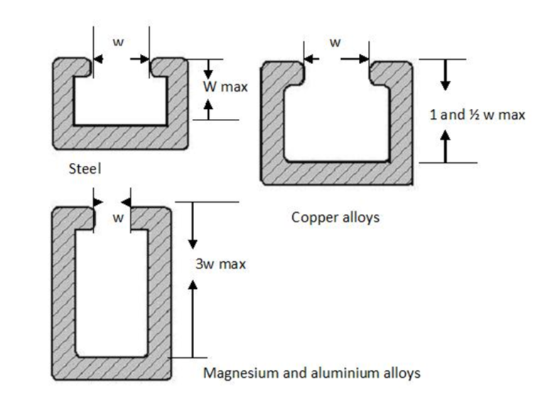
Figure M4.1.9: Design rules for indentations.

• The ratio of length to thickness of any segment should not exceed 14:1. For magnesium it is 20:1 as shown in Figure M4.1.10. 

Figure M4.1.10: The length-to-thickness ratio of any section of an extrusion of steel or other difficult-to-extrude material should not exceed14.

• Symmetrical cross sections are preferable to non-symmetrical designs to avoid unbalanced stresses and warpage. Design recommendation has been shown in the Figure M4.1.11. 

Figure M4.1.11: Nonsymmetrical shape by extruding asymmetrical section and dividing it in two.

Dimensional factor

Extrusion is a hot process and temperature and cooling rate variation affect the final dimension of the extruded parts. Hence, extruded parts are more inherent to piece-to-piece and drawing-topiece dimensional variation than parts made with other processes.         

Recommended tolerances

Table M4.1.2 summarizes the recommended tolerances for extruded parts for ferrous metal.

Table M4.1.2: Recommended Dimensional Tolerances for Ferrous-Metal Extrusions. (Source: Design for Manufacturability Handbook by James G Bralla, 2nd Ed)

Table M4.1.3: Recommended Dimensional Tolerances for Ferrous-Metal Extrusions. (Source: Design for Manufacturability Handbook by James G Bralla, 2nd Ed)

 

HEAT EXCHANGERS -IN BRIEF NOTES

7.1 What are heat exchangers?  

 

Heat exchangers are devices used to transfer heat energy from one fluid to another.  Typical heat exchangers experienced by us in our daily lives include condensers and evaporators used in air conditioning units and refrigerators.  Boilers and condensers in thermal power plants are examples of large industrial heat exchangers. There are heat exchangers in our automobiles in the form of radiators and oil coolers. 

 Heat exchangers are also abundant in chemical and process industries. 

There is a wide variety of heat exchangers for diverse kinds of uses, hence the construction also would differ widely. However, in spite of the variety, most heat exchangers can be classified into some common types based on some fundamental design concepts. We will consider only the more common types here for discussing some analysis and design methodologies.  

7.2 Heat Transfer Considerations 

 The energy flow between hot and cold streams, with hot stream in the bigger diameter tube, is as shown in Figure 7.1.  Heat transfer mode is by convection on the inside as well as outside of the inner tube and by conduction across the tube.  Since the heat transfer occurs across the smaller tube, it is this internal surface which controls the heat transfer process.  By convention, it is the outer surface, termed Ao, of this central tube which is referred to in describing heat exchanger area.  Applying the principles of thermal resistance,

 

Figure 7.1: End view of a tubular heat exchanger

ln Standard convective correlations are available in text books and handbooks for the convective coefficients, ho and hi. The thermal conductivity, k, corresponds to that for the material of the internal tube.  To evaluate the thermal resistances, geometrical quantities (areas and radii) are determined from the internal tube dimensions available.   

7.3 Fouling 

Material deposits on the surfaces of the heat exchanger tubes may add more thermal resistances to heat transfer.  Such deposits, which are detrimental to the heat exchange process, are known as fouling. Fouling can be caused by a variety of reasons and may significantly affect heat exchanger performance.  With the addition of fouling resistance, the overall heat transfer coefficient, Uc, may be modified as:   

" where R” is the fouling resistance. 

Fouling can be caused by the following sources: 

1) Scaling is the most common form of fouling and is associated with inverse solubility salts.  Examples of such salts are CaCO3, CaSO4, Ca3(PO4)2, CaSiO3, Ca(OH)2, Mg(OH)2, MgSiO3, Na2SO4, LiSO4, and Li2CO3.   2) Corrosion fouling is caused by chemical reaction of some fluid constituents with the heat exchanger tube material. 

 3) Chemical reaction fouling involves chemical reactions in the process stream which results in deposition of material on the heat exchanger tubes. This commonly occurs in food processing industries.

 4) Freezing fouling is occurs when a portion of the hot stream is cooled to near the freezing point for one of its components.  This commonly occurs in refineries where paraffin frequently solidifies from petroleum products at various stages in the refining process. , obstructing both flow and heat transfer.

 5) Biological fouling is common where untreated water from natural resources such as rivers and lakes is used as a coolant.  Biological microorganisms such as algae or other microbes can grow inside the heat exchanger and hinder heat transfer. 

6) Particulate fouling results from the presence of microscale sized particles in solution.  When such particles accumulate on a heat exchanger surface they sometimes fuse and harden. Like scale these deposits are difficult to remove. 

 With fouling, the expression for overall heat transfer coefficient becomes:

7.4 Basic Heat Exchanger Flow Arrangements 

Two basic flow arrangements are as shown in Figure 7.2.  Parallel and counter flow provide alternative arrangements for certain specialized applications.  In parallel flow both the hot and cold streams enter the heat exchanger at the same end and travel to the opposite end in parallel streams.  Energy is transferred along the length from the hot to the cold fluid so the outlet temperatures asymptotically approach each other.  In a counter flow arrangement, the two streams enter at opposite ends of the heat exchanger and flow in parallel but opposite directions.  Temperatures within the two streams tend to approach one another in a nearly linearly fashion resulting in a much more uniform heating pattern.  Shown below the heat exchangers are representations of the axial temperature profiles for each.  Parallel flow results in rapid initial rates of heat exchange near the entrance, but heat transfer rates rapidly decrease as the temperatures of the two streams approach one another. This leads to higher exergy loss during heat exchange. Counter flow provides for relatively uniform temperature differences and, consequently, lead toward relatively uniform heat rates throughout the length of the unit.

 Fig. 7.2 Basic Flow Arrangements for Tubular Heat Exchangers.   

7.5 Log Mean Temperature Differences 

Heat flows between the hot and cold streams due to the temperature difference across the tube acting as a driving force.  As seen in the Figure 7.3, the temperature difference will vary along the length of the HX, and this must be taken into account in the analysis. 

Fig. 7.3 Temperature Differences Between Hot and Cold Process Streams 

 From the heat exchanger equations shown earlier, it can be shown that the integrated average temperature difference for either parallel or counter flow may be written as: 

The effective temperature difference calculated from this equation is known as the log mean temperature difference, frequently abbreviated as LMTD, based on the type of mathematical average that it describes.  While the equation applies to either parallel or counter flow, it can be shown that eff will always be greater in the counter flow arrangement.   

 Another interesting observation from the above Figure is that counter flow is more appropriate for maximum energy recovery.  In a number of industrial applications there will be considerable energy available within a hot waste stream which may be recovered before the stream is discharged.  This is done by recovering energy into a fresh cold stream.  Note in the Figures shown above that the hot stream may be cooled to t1 for counter flow, but may only be cooled to t2 for parallel flow.  Counter flow allows for a greater degree of energy recovery.  Similar arguments may be made to show the advantage of counter flow for energy recovery from refrigerated cold streams.  

7.6 Applications for Counter and Parallel Flows

       We have seen two advantages for counter flow, (a) larger effective LMTD and (b) greater potential energy recovery.  The advantage of the larger LMTD, as seen from the heat exchanger equation, is that a larger LMTD permits a smaller heat exchanger area, Ao, for a given heat transfer, Q.  This would normally be expected to result in smaller, less expensive equipment for a given application.    Sometimes, however, parallel flows are desirable (a) where the high initial heating rate may be used to advantage and (b) where it is required the temperatures developed at the tube walls are moderate.  In heating very viscous fluids, parallel flow provides for rapid initial heating and consequent decrease in fluid viscosity and reduction in pumping requirement.  In applications where moderation of tube wall temperatures is required, parallel flow results in cooler walls. This is especially beneficial in cases where the tubes are sensitive to fouling effects which are aggravated by high temperature.  

7.7 Multipass Flow Arrangements

In order to increase the surface area for convection relative to the fluid volume, it is common to design for multiple tubes within a single heat exchanger.    

With multiple tubes it is possible to arrange to flow so that one region will be in parallel and another portion in counter flow.  An arrangement where the tube side fluid passes through once in parallel and once in counter flow is shown in the Figure 7.4.  Normal terminology would refer to this arrangement as a 1-2 pass heat exchanger, indicating that the shell side fluid passes through the unit once, the tube side twice.  By convention the number of shell side passes is always listed first.  

                                         Fig. 7.4 Multipass flow arrangement  

The primary reason for using multipass designs is to increase the average tube side fluid velocity in a given arrangement.  In a two pass arrangement the fluid flows through only half the tubes and any one point, so that the Reynold’s number is effectively doubled.  Increasing the Reynolds’s number results in increased turbulence, increased Nusselt numbers and, finally, in increased convection coefficients.  Even though the parallel portion of the flow results in a lower effective T, the increase in overall heat transfer coefficient will frequently compensate so that the overall heat exchanger size will be smaller for a specific service.  The improvement achievable with multipass heat exchangers is substantialy large. Accordingly, it is a more accepted practice in modern industries compared to conventional  true parallel or counter flow designs.  The LMTD formulas developed earlier are no longer adequate for multipass heat exchangers.  Normal practice is to calculate the LMTD for counter flow, LMTDcf, and to apply a correction factor, FT, such that 

The correction factors, FT, can be found theoretically and presented in analytical form.  The equation given below has been shown to be accurate for any arrangement having 2, 4, 6, .....,2n tube passes per shell pass to within 2%. 

where the capacity ratio, R, is defined as:

The effectiveness may be given by the equation: 

7.8 Effectiveness-NTU Method:

Quite often, heat exchanger analysts are faced with the situation that only the inlet temperatures are known and the heat transfer characteristics (UA value) are known, but the outlet temperatures have to be calculated. Clearly, LMTH method will not be applicable here. In this regard, an alternative method known as the ε-NTU method is used.  Before we introduce this method, let us ask ourselves following question: conditions ?Exchange  perform  for  given inlet How  will  existing  Heat ness:

Define effectiveness

 The effectiveness, ε, is the ratio of the energy recovered in a HX to that recoverable in an ideal HX. 

 

NTUmax can be obtained from figures in textbooks/handbooks    First, however, we must determine which fluid has Cmin. 

ABS - ANTI BRAKE LOCKING SYSTEM

Anti-Lock Braking System (ABS)

The ABS (Anti-lock Brake System) monitors the speed of each wheel to detect locking. When it detects sudden braking, it will release braking pressure for a moment and then provide optimum braking pressure to each wheel. By repeating this process in a short period of time, it enhances steering control during sudden stops. As a result, it will also help improve the ability of stopping the vehicle.

ABS only supports the driver's control of the vehicle, and it is not a substitute for it. It is the driver's responsibility to drive at the appropriate speed depending on the condition of the road and to keep a generous distance from the car ahead of you.

Supports unexpected braking in case of emergency
Studies show that nearly half of all drivers do not step on the brake quickly and strongly enough to stop the vehicle in case of an emergency 

When Brake Assist detects an attempted panic stop, it supports drivers by strengthening the power
Brake Assist will detect attempted panic braking based on the force that is applied to the brake pedal and how fast the driver is stepping on the pedal. When the system recognizes sudden braking, it will add additional pressure to the brake.

When your foot is released during Braking Assist,braking power lessens and regulates the brakes with ease.

Traction Control (TRC)

When you are starting the vehicle or accelerating on a wet surface, you could lose control of the wheel because of wheel spin. TRC will help prevent such events from happening.

TRC continually monitors the condition between the tires and the surface of the road.When it detects wheel spin, the system applies brakes or slows down the engine to regulate spinning and help ensure proper contact of tires. This help prevent the car from becoming unstable.

There might be the cases in which the half-side of the wheel runs off or the wheels spin off on the snowy road. And also there might be the case that the current tractino control might not be working well.In those cases, Auto LSD is one of the technologies which both improve startability and runability.

Purpose

Anti-lock brake systems (ABS) - generally also referred to as anti-lock systems (ALS) - are designed to prevent the vehicle wheels from locking as a result of the service brake being applied with too much force, especially on slippery road surfaces.

The idea is to maintain cornering forces on braked wheels to ensure that

the vehicle or vehicle combination retains its drivin

g stability and manoeuvrability as far as physically possible. The available powertransmission or grip between tyres and carriageway should also be utilised as

far as possible to minimise the braking distance and maximise vehicle deceleration.

Why ABS?

Although today commercial vehicle brakes are designed to a very hightechnical standard, braking on slippery roads often results in potentially dangerous situations. During full or even partial braking on a slippery road it may no longer be possible to fully transfer the braking force onto the road due to the low coefficient of friction  (friction coefficient (k)) between the tyres and the carriageway. The braking force is excessive and the wheels lock up. Locked wheels no longer provide any grip on the

road and are almost incapable of transferring any cornering forces (steering and tracking forces).

This often has dangerous consequences:

– The vehicle becomes unsteerable

– The vehicle breaks away in spite of countersteering, and starts to swerve.

– The braking distance is significantly increased

– Tractor-trailer combinations or semitrailer trains may break away or jackknife.

Load sensing valve influence

On dry roads today’s load sensing valves (ALB) alone are often capable of preventing the wheels from locking if the vehicle is unladen; they also help the driver to effectively grade the braking process on wet road surfaces, but they are unable to prevent locking as such (no slip monitoring). In addition, they are unable to counteract any overreactions on the part of the driver, or any variances in frictional or adhesion coefficients which may apply to different sides of the vehicle, or indeed to its different axles (μ split road surfaces).

Benefits of ABS:

Only the Anti-Lock Brake System (ABS)

– guarantees stable braking characteristics on all road surfaces.

– maintains steerability and generally reduces the braking distance

– prevents vehicle combinations from jackknifing

– reduces tyre wear.

Limits of ABS

Although ABS is an effective safety device, it can not suspend the limits

defined by driving physics. Even a vehicle fitted with ABS will become uncontrollable if driven too fast around a corner. So ABS is not a licence for a maladjusted style of driving or failure to observe the correct safety distance.

automotive store